Distributed Processing
Description
The distributed processing module is designed to solve the problem of efficient processing for large-scale point clouds that cannot be handled by a single computer. It supports multi-node collaboration for processing large-volume point cloud data.
Workflow
Assume that four computers are available: one computer is used as the master node, and the other three computers are used as computing nodes.
1. Set Up and Start Each Computing Node
Start LiDAR360 on multiple independent computers and click the Start Computing Node button on the main page. The Computing Node Settings dialog box is displayed, as shown below.
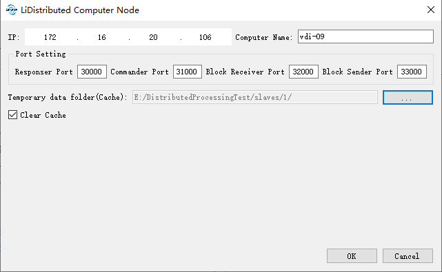
In this dialog box, enter the IP address of the current computer and each port number. In general, the default port numbers can be used. After clicking OK, the Computing Node Monitor dialog box is displayed, as shown below.
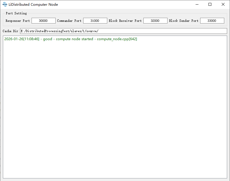
The list at the bottom of the dialog box displays the running log of the current computing node in real time.
2. Set Up and Start the Master Node
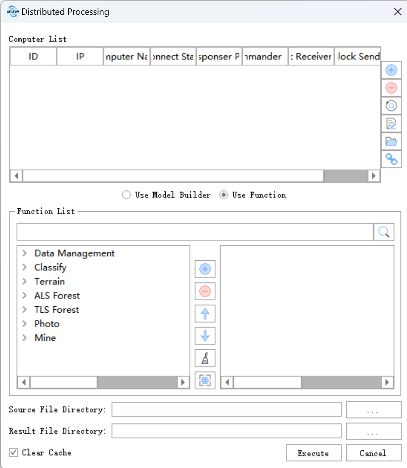
After all computing nodes have been started and configured, click the Distributed Computing button on the LiDAR360 main page. The Master Node Settings dialog box is displayed, as shown below.
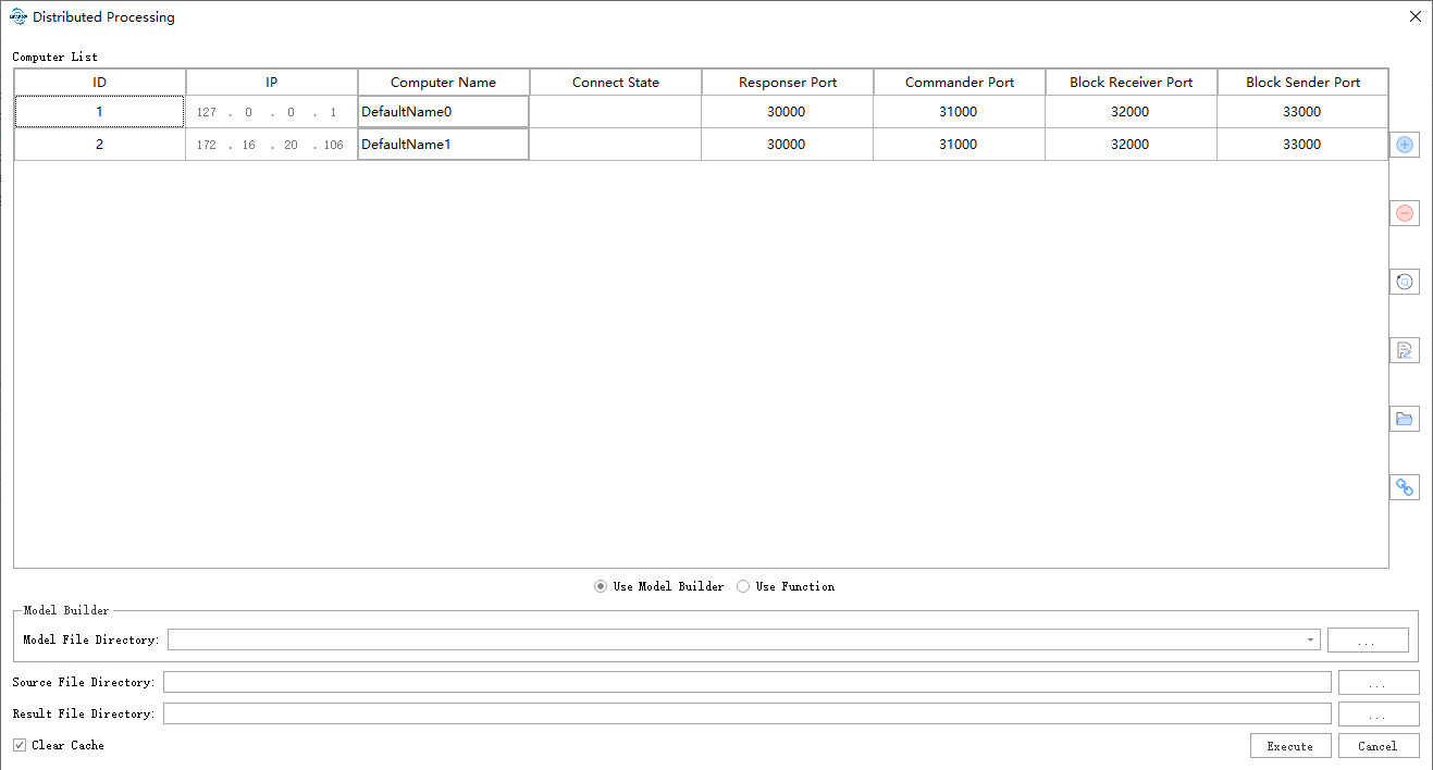
The Master Node Settings dialog box is used to configure distributed tasks. The configuration mainly includes the following five parts.
(1) Configure the IP Address and Port Number of Each Computing Node
The upper part of the Master Node Settings dialog box is the computing node configuration area. The IP address and port number configured here must be the same as those entered in the Computing Node Settings dialog box described above.
(2) Automatically Search for Computing Nodes
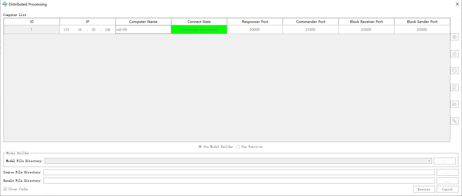
Click Query Nodes in the Master Node Settings dialog box to automatically search for online computing nodes, as shown below.
(3) Configure Computing Tasks
The middle part of the Master Node Settings dialog box is the computing task configuration area. Configure the tasks that need distributed processing in the function list.
(4) Set Source and Result Point Cloud Directories
The source point cloud directory and result point cloud directory are configured in the lower-middle part of the Master Node Settings dialog box. The source point cloud directory stores the point cloud data to be processed and can contain multiple large point cloud files. The distributed processing results are finally output to the result point cloud directory.
(5) Set the Model Builder File Path
Distributed computing supports parsing and processing model files saved by the Model Builder module. Enter the model file to be processed in this section.
The following figure shows an example distributed computing task configuration. The example contains one computing node with the IP address 192.168.20.102, and the computing tasks include Remove Outliers and Noise Filter.
3. Start the Distributed Computing Workflow
Click Execute in the Master Node Settings dialog box. The Master Node Monitor dialog box is displayed and the distributed computing workflow starts.
Monitoring Distributed Tasks
After the distributed computing workflow starts, the Master Node Monitor dialog box is displayed, as shown below.
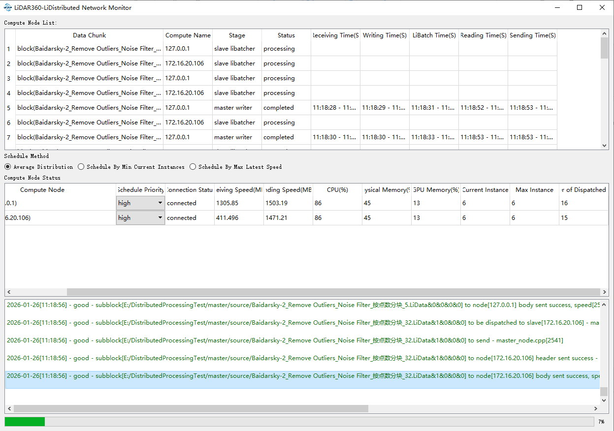
In the Master Node Monitor interface, the upper list displays real-time information about each source point cloud block, including the IP address of the computing node to which the block is scheduled, the current stage of the block, the current status of the block, and the time consumed for computing the block. Below the source point cloud block list is the task scheduling method for the current distributed computing task. Two scheduling strategies are provided for real-time selection: Minimum Current Computing Instance Count and Maximum Processing Speed. The list below the scheduling method area displays real-time information about each computing node, including connection status, point cloud transfer speed, CPU usage, memory usage, the current number of Libatch instances running on the computing node, and the historical maximum number of Libatch instances running on the computing node. The bottom of the Master Node Monitor interface is the log output area and the overall progress information for distributed computing.
Distributed Workflow for Image Aerial Triangulation
Image aerial triangulation (alignment) also supports distributed operation. It is different from the point cloud workflow. Image distributed processing depends on LAN communication and shared file storage. Data is no longer distributed to each node; instead, distributed processing is implemented by directly reading and writing data in a shared folder.
Minimum Device Requirements for Image Distributed Nodes
| Item | Minimum Requirement |
|---|---|
| Quantity | 2 or more computers |
| Operating System | Windows 10 or later |
| Memory | 32 GB or higher |
| Graphics Card | NVIDIA RTX 1660 or higher |
| Disk | Mechanical hard disk with 500 GB or more free storage |
Shared Folder Configuration
The shared folder is mainly used to store raw data and result files.
- Right-click the disk or folder to be shared, select Properties, and open the folder properties window.
- Click the Sharing tab, and click Share under Network Path to open the sharing settings interface.
- In the pop-up interface, select the user name that should have access to the shared folder.
- Grant the user read/write permission in the permission column.
- Click Share to complete folder sharing.
Path access rules:
| Method | Recommendation | Description |
|---|---|---|
IP + path, such as \\192.168.1.10\share\project |
Recommended | Stable and reliable |
| Computer name + path | Alternative | Depends on DNS resolution |
Mapped network drive, such as Z:\project |
Not recommended | Local unmapped drive letters are not recommended |
How to Call Image Distributed Processing
As shown below:
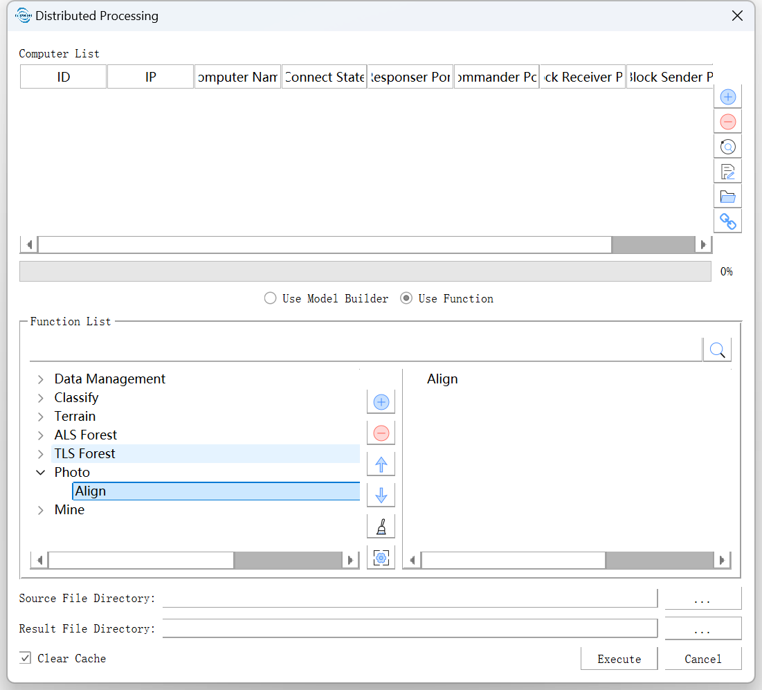
Select the function to use and click Image Alignment. The source file directory must contain the image projects to be processed in distributed mode. All image projects in this path are included in the distributed operation.